Stationarity and Decomposition

Outlier Exploration

Outliers have influence on the model training procedure, as the model could incorporate these outliers unless they are eliminated. Figure 1 provides a broad overview of outliers within the context of monthly and quarterly aggregated data.

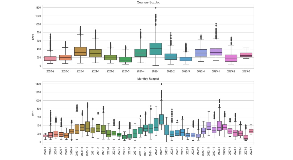
Figure 1: Outliers overview.

The boxplots presented in Figure 1 offer an effective way of visualizing the underlying seasonality and trend patterns within the dataset which we will explore in the next section. While our time series exhibits outliers, these instances correspond to exceptionally high wave heights and appear unrelated to errors or undesired circumstances. Consequently, we have opted to allow our training model to incorporate these outliers. Nevertheless, we have retained the code responsible for detecting and eliminating outliers, preserving it for potential future explorations.

Data Stationarity

The importance of this step depends on the choice of our prediction model. While certain statistical models adeptly manage non-stationary data, the majority of machine learning models perform optimally with time series that exhibit stationarity, wherein both seasonality and trend components are eliminated. Since we intend to forecast this series using a machine learning methodology, this segment entails an assessment of the dataset's stationarity and removing any components that disrupt stationarity.

An effective approach for assessing the stationarity of a series is through visualization. As depicted in Figure 8, the SWH series is presented for our target station across each year. Observing the graphs, it becomes apparent that the series experiences higher fluctuations (higher standard deviation) during the initial and ending months of the year, during the cold seasons. Aside from this annual cyclic pattern, no distinct minor seasonal trends are evident in the plot. It's possible that there are more complex patterns of seasonality hidden within the dataset.

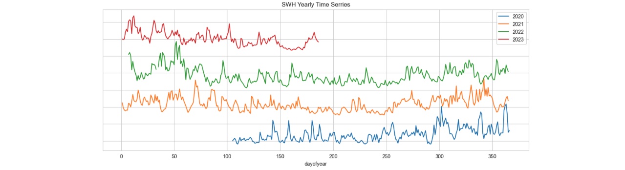
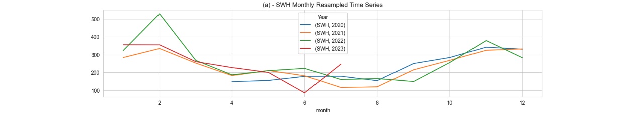
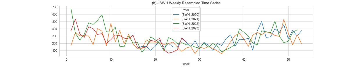
Figure 2: SWH presented for target station "AMETS Berth B Wave Buoy" across each year with different resampling size.

We examined different methodology to detect more seasonality component in the series including weekly, 29.5 days (moon cycle period), monthly, and quarterly but we did not find any rhythmic seasonality. Among the methodologies that we experimented with, we can mention STL, seasonal_decompose, as well as ACF and PACF plots. Coding details of these efforts are available in my Github. We found satisfaction in utilizing the annual seasonal and trend components identified by STL (Seasonal-Trend Decomposition using Loess), given that it has yielded a successful prediction model for this project.

To remove the yearly seasonal component, we applied the STL method to both the original dataset with a 10-minute interval and a resampled dataset with 1-hour frequency. The outcomes were almost identical for both cases. However, it's worth noting that the execution time for the STL method was significantly longer with the 10-minute interval data (6 times larger data size). Moreover, the performance of the machine learning model remained consistent regardless of the data frequency. Due to these observations, we opted to proceed with the 1-hour frequency for the duration of this project.

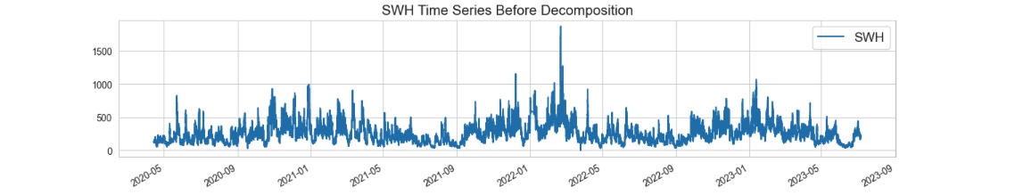
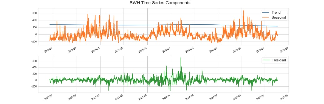
Figure 3: Seasonal, trend, and residual components. Once the seasonal and trend components have been eliminated,
the residuals exhibit a random pattern, indicating that the series can now be considered stationary.

As previously stated, we employed STL to break down our SWH time series. We conducted STL training over a yearly cycle, resulting in the identification of its trend, seasonal, and residual components, as depicted in figure 3. Ultimately, we will proceed to train an XGBoost model using the residuals, which appear to be random and stationarity.

In the next section you can read about the XGBoost model trained to forecast the future of the SWH time series.